What Does It Mean to Just Be Left Continuous
In the previous post I started by introducing the concept of a stochastic process, and their modifications. It is necessary to introduce a further concept, to represent the information available at each time. A filtration 


Given a filtration, its right and left limits at any time and the limit at infinity are as follows
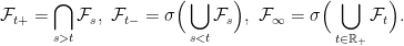
Here, 


A probability space 


Often, in stochastic process theory, filtered probability spaces are assumed to satisfy the usual conditions, meaning that it is complete and the filtration is right-continuous. Note that any filtered probability space can be completed simply by completing the underlying probability space and then adding all zero probability sets to each 
Throughout these notes I assume a complete filtered probability space, although many of the results can be extended to the non-complete case without much difficulty. However, for the sake of a bit more generality, I don't assume that filtrations are right-continuous.
One reason for using filtrations is to define adapted processes. A stochastic process process 


As mentioned in the previous post, it is often necessary to impose measurability constraints on a process 
Definition 1
The most important of these definitions, at least in these notes, is that of predictable processes. While adapted right-continuous processes will be used extensively, there is not much need to generalize to optional processes. Similarly, progressive measurability isn't used a lot except in the context of adapted right-continuous (and therefore optional) processes. On the other hand, predictable processes are extensively used as integrands for stochastic integrals and in the Doob-Meyer decomposition, and are often not restricted to the adapted and left-continuous case.
Given any set of real-valued functions on a set, which is closed under multiplication, the set of functions measurable with respect to the generated sigma-algebra can be identitified as follows. They form the smallest set of real-valued functions containing the generating set and which is closed under taking linear combinations and increasing limits. So, for example, the predictable processes form the smallest set containing the adapted left-continuous processes which is closed under linear combinations and such that the limit of an increasing sequence of predictable processes is predictable.
Another way of defining predictable processes is in terms of continuous adapted processes.
Lemma 2 The predictable sigma-algebra is generated by the continuous and adapted processes.
Proof: Clearly every continuous adapted process is left-continuous and, therefore, is predictable. Conversely, if
Continuity of 


A further method of defining the predictable sigma-algebra is in terms of simple sets generating it. The following is sometimes used.
Lemma 3 The predictable sigma-algebra is generated by the sets of the form
![\displaystyle \left\{(s,t]\times A\colon t>s\ge 0, A\in\mathcal{F}_s\right\}\cup\left\{\{0\}\times A\colon A\in\mathcal{F}_0\right\}.](https://s0.wp.com/latex.php?latex=%5Cdisplaystyle++%5Cleft%5C%7B%28s%2Ct%5D%5Ctimes+A%5Ccolon+t%3Es%5Cge+0%2C+A%5Cin%5Cmathcal%7BF%7D_s%5Cright%5C%7D%5Ccup%5Cleft%5C%7B%5C%7B0%5C%7D%5Ctimes+A%5Ccolon+A%5Cin%5Cmathcal%7BF%7D_0%5Cright%5C%7D.+&bg=ffffff&fg=000000&s=0&c=20201002)
(1)
Proof: If 


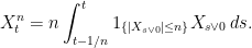
Conversely, let X be left-continuous and adapted. Then it is the limit of the piecewise constant functions

as n goes to infinity. Each of the summands on the right hand side is easily seen to be measurable with respect to the sigma-algebra generated by the collection (1). So, 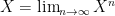
In these notes, I refer to the collection of finite unions of sets in the collection (1) as the elementary or elementary predictable sets. Writing these as 

Finally, the different forms of measurability can be listed in order of generality, starting with the predictable processes, up to the much larger class of jointly measurable adapted processes.
Lemma 4 Each of the following properties of a stochastic process implies the next
- predictable.
- optional.
- progressive.
- adapted and jointly measurable.
Proof: As the predictable sigma-algebra is generated by the continuous adapted processes, which are also optional by definition, it follows that all predictable processes are optional.
Now, if 


Finally, consider a progressively measurable process 
![{[0,t]\times\Omega}](https://s0.wp.com/latex.php?latex=%7B%5B0%2Ct%5D%5Ctimes%5COmega%7D&bg=ffffff&fg=000000&s=0&c=20201002)
![{\mathcal{B}([0,t])\otimes\mathcal{F}_t}](https://s0.wp.com/latex.php?latex=%7B%5Cmathcal%7BB%7D%28%5B0%2Ct%5D%29%5Cotimes%5Cmathcal%7BF%7D_t%7D&bg=ffffff&fg=000000&s=0&c=20201002)

stallardsuplusentep.blogspot.com
Source: https://almostsuremath.com/2009/11/08/filtrations-and-adapted-processes/
0 Response to "What Does It Mean to Just Be Left Continuous"
Postar um comentário